Making movies in R

Overview

I often work with data that vary in both time and space. Underwater gliders, for example, move around as they explore the ocean for weeks to months at a time. The ocean they observe changes depending on where they go, and when they go there. This ‘spatiotemporal variation’ is often important to understand, but can be very difficult to visualize with typical static plots. Movies can help. This post outlines a quick means of producing a movie from plots created in R.

Data

For this example, I chose to create a simple ‘gif’ movie of the track of Captain Cook’s voyage around the world on the HMS Endeavor. The data are available in the ocedata package. Here’s a quick look at the data:

library(oce)
library(ocedata)
data(coastlineWorld)
data(endeavour)

# summary of the endeavour dataset
summary(endeavour)
##       time                        latitude         longitude      
##  Min.   :1768-08-26 00:00:00   Min.   :-60.067   Min.   :-178.02  
##  1st Qu.:1769-01-06 18:00:00   1st Qu.:-35.746   1st Qu.:-118.09  
##  Median :1769-08-21 12:00:00   Median :-22.767   Median : -37.95  
##  Mean   :1769-12-11 14:40:52   Mean   :-14.465   Mean   : -48.98  
##  3rd Qu.:1771-02-28 06:00:00   3rd Qu.:  4.908   3rd Qu.: -10.68  
##  Max.   :1771-07-10 00:00:00   Max.   : 49.500   Max.   : 175.35

# plot full track
mapPlot(coastlineWorld, proj='+proj=moll', col='lightgray')
mapPoints(endeavour$longitude, endeavour$latitude, pch=20, cex=2/3, col='red')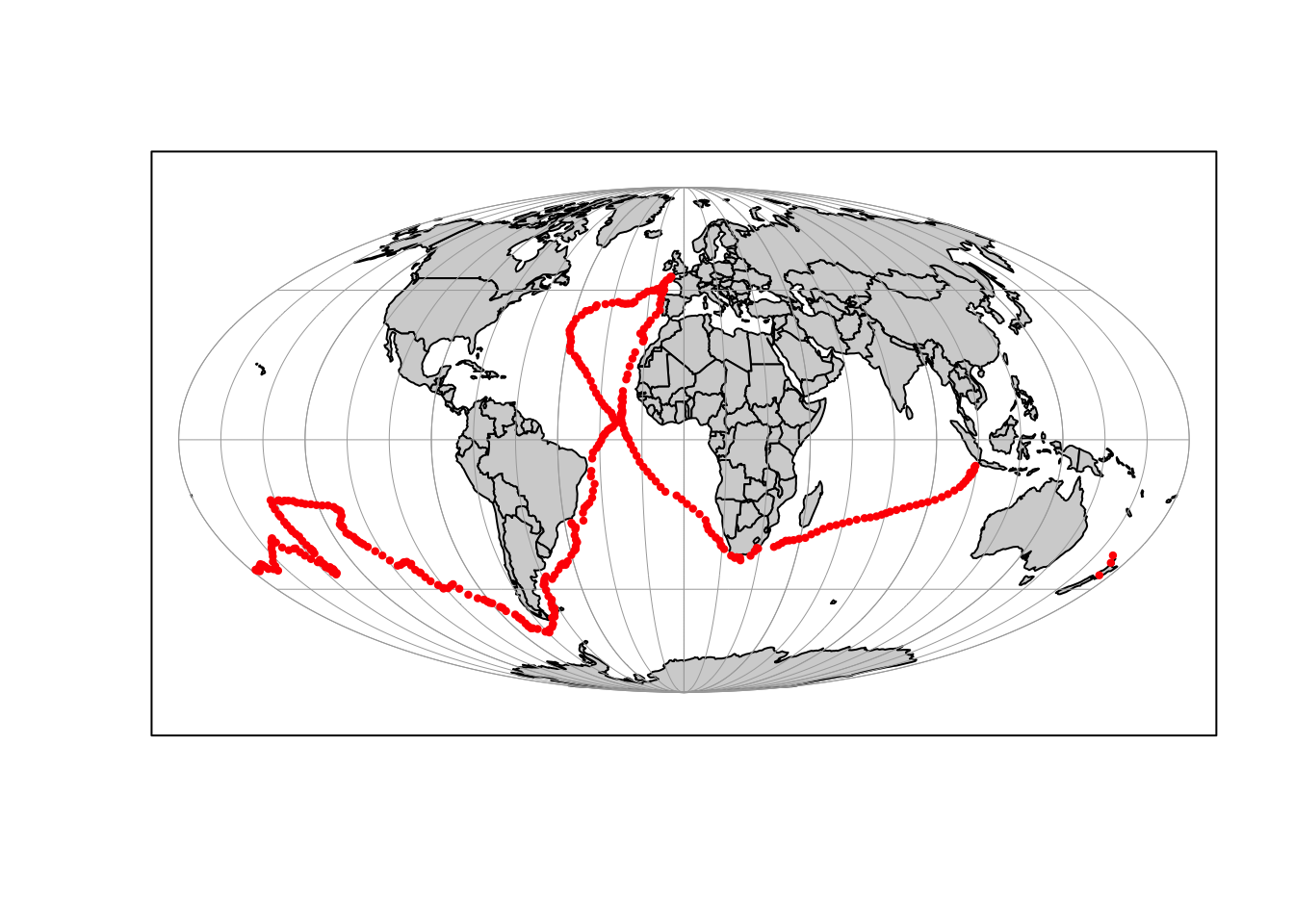

This kind of static map provides a nice global overview, but doesn’t give a great sense of how that the voyage progressed over time.

Step 1: make many plots

The next step is to generate timesteps spanning the entire voyage, then create a map of the ship track during each timestep and save it to a temporary file. I chose a month long timestep to keep the numbers of plots reasonable. For the sake of concision the output (i.e. all 35 plots) is not shown in this post. I got a little fancy here and decided to use an orthographic map projection, but you could use just about any projection you like. It’s also worth noting again that this approach would work for any type of plot, not just maps.

# input parameters
map_dir = 'figures' # directory for temporary maps
outfile = 'static/movie.gif' # movie file (this could be several different file types)
movie_speed = 5 # movie play speed

# rename data
df = endeavour

# make maps ---------------------------------------------------------------
if(!dir.exists(map_dir)){dir.create(map_dir)}

# start and end times
t0 = min(df$time)
t1 = max(df$time)

# time vector
tseq = seq.POSIXt(t0, t1+31*60*60*24, by = 'month')

# make and save maps
for(it in 1:(length(tseq)-1)){
  
  # subset within timestep
  it0 = tseq[it]
  it1 = tseq[it+1]
  idf = df[df$time >= it0 & df$time <= it1,]
  
  # open map file
  png(paste0(map_dir,'/', as.character(format(it0, '%Y-%m-%d.png'))), 
      width=6, height=6, unit="in", res=175, pointsize=10)
  
  # center map (only if ship moved)
  if(nrow(idf)!=0){
    mlat = idf$latitude[which.max(idf$time)]
    mlon = idf$longitude[which.max(idf$time)]
    p = paste0("+proj=ortho +lat_0=", mlat, " +lon_0=", mlon)  
  }
  
  # plot
  mapPlot(coastlineWorld, col = 'lightgrey', projection = p)
  
  # plot entire track
  mapPoints(df$longitude,df$latitude, pch = 16, col = 'grey', cex = 1/3)
  
  # add current section
  mapPoints(idf$longitude,idf$latitude, pch = 16, col = 'blue', cex = 2/3)
  
  # add latest
  mapPoints(mlon,mlat, pch = 21, bg = 'red', cex = 1)
  
  # add timestamp
  mtext(text = paste0(format(it1, '%b, %Y')), side = 3, line = 0, adj = 0)
  
  # start message
  if(it==1){
    title('Start!')
  }
  
  # end message
  if(it==length(tseq)-1){
    title('Done!')
  }
  
  # close and save plot
  dev.off()
  
}

Step 2: stitch plots into movie

Now you should have a directory full of monthly maps. The final step is to stitch all these maps together into a movie. In this case we’re making a ‘gif’, but it can be any number of types of movie files. The way I do this requires us to step outside R and use the imagemagick command line tool. If you have a mac, imagemagick is easily installed with the homebrew package manager using the command brew install imagemagick (see the full formula here). The segment below assembles a system command to execute imagemagick’s convert function from within R, then deletes the directory with all the temporary figures.

# write system command
cmd = paste0('convert -antialias -delay 1x', movie_speed, ' ', map_dir, '/*.png ', outfile)

# execute system command
system(cmd)

# remove temporary files
unlink(map_dir, recursive = T)

There it is! It’s not perfect, but it shows the voyage with an extra level of detail not available or obvious in the static map. Now we can see, for example, that he hung out for awhile in New Zealand (while charting the coast), and that we’re missing some data for his transit up the coast of Australia. It’s a simple example, but hopefully demonstrates the approach and how it may be refined or tweaked to work with other datasets.