I put together a few R tutorials recently, and ended the series with a quick tutorial of how to download and plot satellite-derived sea surface temperature (SST) data in R. Well, I thought it would be quick. It took me longer than I expected to figure out. Now that I have, though, I’m happy with the result and thought others might be interested as well. If nothing else, you can make some very pretty pictures.
The satellite data I’m using aren’t strictly satellite data. It’s actually a product from NOAA called the ‘optimum interpolation sea surface temperature’ (OISST) dataset, which is a compilation of satellite and other remote-sensed data. It’s updated daily, has global coverage with 1/4 degree resolution, and extends all the way back to 1981. Most importantly, it’s freely available to download! You can learn more at the NOAA website.
Setup
Begin by selecting the date to plot, then read in a few libraries for plotting (oce, and ocedata) and working with netcdf files that contain the satellite data (ncdf4). Users on windows machines may have issues with the ncdf4 library, but apparently these issues have been resolved in recent package upgrades.
# libraries
suppressPackageStartupMessages(library(oce))
suppressPackageStartupMessages(library(ncdf4))
suppressPackageStartupMessages(library(ocedata))
data("coastlineWorld")

# choose date
dt = as.Date('2018-09-17')
Download and format the data
The next step is to download and format the data. This involves 1) creating a url to the data, 2) downloading the file if you haven’t done so already, and 3) extracting relevant data from the downloaded netcdf file.
# convert date to new format
dt = format(dt, '%Y%m%d')

# assemble url to query NOAA database
url_base = paste0("https://www.ncei.noaa.gov/data/sea-surface-temperature-optimum-interpolation/access/", dt, "120000-NCEI/0-fv02/")
data_file = paste0(dt, "120000-NCEI-L4_GHRSST-SSTblend-AVHRR_OI-GLOB-v02.0-fv02.0.nc")

# define data url
data_url = paste0(url_base, data_file)

# download netcdf
if(!file.exists(data_file)){
  download.file(url = data_url, destfile = data_file)
} else {
  message('SST data already downloaded! Located at:\n', data_file)
}

# open netcdf file and extract variables
nc = nc_open(data_file)

# view netcf metadata
# print(netcdf)

# extract data
lat = ncvar_get(nc, "lat")
lon = ncvar_get(nc, "lon")
time = ncvar_get(nc, "time")
sst = ncvar_get(nc, "analysed_sst")

# close netcdf
nc_close(nc)

# convert timestamp
time = as.POSIXct(time, origin = '1981-01-01 00:00:00', tz = 'UTC')

# convert units from kelvin to celcius
sst = sst - 273.15
Plot data
Last step is to plot the data. This requires us to configure the plot window to plot both the map and a colorbar alongside. After that, we simply rely on the sweet tools built by the oce developers to plot a nice make of global SST.
# setup layout for plotting
m = rbind(
  c(1,1,1,1,1,1,1,1,1,1,1,2),
  c(1,1,1,1,1,1,1,1,1,1,1,2),
  c(1,1,1,1,1,1,1,1,1,1,1,2),
  c(1,1,1,1,1,1,1,1,1,1,1,2),
  c(1,1,1,1,1,1,1,1,1,1,1,2),
  c(1,1,1,1,1,1,1,1,1,1,1,2)
)

layout(m)

# configure colour scale for plotting
pal = oce.colorsTemperature()
zlim = range(sst, na.rm = TRUE)
c = colormap(sst, breaks=100, zclip = T, col = pal, zlim = zlim)

# define unit label
lab = 'Optimum Interpolation SST [deg C]'

# plot basemap
plot(coastlineWorld, col = 'grey',
     projection = "+proj=eck3",
     longitudelim=range(lon),
     latitudelim=range(lat))

# add sst layer
mapImage(lon, lat, sst, col=oceColorsTemperature)

# overlay coastline again
mapPolygon(coastlineWorld, col='grey')

# add variable label
mtext(paste0(lab),side = 3, line = 0, adj = 0, cex = 0.7)

# add title
title(paste0(time))

# add colour palette
drawPalette(c$zlim, col=c$col, breaks=c$breaks, zlab = '', fullpage = T)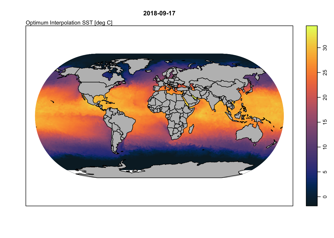
That’s it! Happy plotting :)